Recipes

Short code for common tasks. Each recipe runs on its own, on the simulation that ships with the repository and is executed when this documentation is built. The Tutorial notebooks work through the same tasks at length.

Every recipe starts from the sample folder:

from pathlib import Path

import numpy as np
import grand

SAMPLE = (Path(grand.__file__).parents[1]
          / "sim2root/Common/sim_Xiaodushan_20221026_000000_RUN1_CD_ZHAireS_0000")

Every event of a folder 

EventList joins the run, shower and trace trees into one event object:

from grand.aoi.event_list import EventList

for event in EventList(str(SAMPLE)):
    shower = event.simshower
    print("event %5d: zenith %5.2f deg, energy %.2g GeV, %2d antennas"
          % (event.event_number, shower.zenith, shower.energy_primary,
             len(event.antennas)))

event 13790: zenith 79.43 deg, energy 3.9e+09 GeV, 44 antennas
event  1618: zenith 51.64 deg, energy 3.8e+09 GeV,  5 antennas

EventList reuses one Event object for every event. To keep values across iterations, copy them out, as above, rather than storing event.

All the trees of a folder 

DataDirectory opens every file of a folder and gives each tree as an attribute, by type and analysis level:

from grand.dataio import DataDirectory

folder = DataDirectory(str(SAMPLE))
tshower = folder.tshower_l0
tshower.get_entry(0)
print("primary %s (PDG code), Xmax %.1f g/cm2" % (tshower.primary_type, tshower.xmax_grams))

primary 2212 (PDG code), Xmax 794.6 g/cm2

A bare attribute, such as folder.tefield, gives the highest level present.

Many files without memory growth 

Release each tree when you are done with it. The with form does it even if the loop raises. Here, every ADC file of the simulations in the repository:

from grand.dataio import TADC

n_events = 0
for path in sorted(SAMPLE.parent.glob("sim_*/adc_*.root")):
    with TADC(str(path)) as tadc:
        for event, run in tadc.get_list_of_events():
            tadc.get_event(event, run)
            n_events += 1               # your analysis of one event goes here
print(n_events, "events read")

15 events read

The antennas in latitude and longitude 

Antenna positions are stored in meters in the array frame (x north, y west, z up) around the run’s origin. Convert them to geodetic coordinates:

from grand import Geodetic, GRANDCS
from grand.dataio import TRun

with TRun(str(SAMPLE / "run_1_L0_0000.root")) as trun:
    trun.get_entry(0)
    xyz = np.asarray(trun.du_xyz)                  # (units, 3), in m
    lat0, lon0, h0 = np.asarray(trun.origin_geoid)

origin = Geodetic(latitude=lat0, longitude=lon0, height=h0)
antennas = Geodetic(GRANDCS(x=xyz[:, 0], y=xyz[:, 1], z=xyz[:, 2], location=origin))
lat, lon, height = np.asarray(antennas)
print("%d antennas, latitude %.3f to %.3f, longitude %.3f to %.3f"
      % (len(lat), lat.min(), lat.max(), lon.min(), lon.max()))

49 antennas, latitude 40.975 to 41.060, longitude 93.857 to 94.005

The geomagnetic field and the geoid at a site 

from grand.geo.geomagnet import field
from grand.geo.topography import geoid_undulation

b = np.asarray(field(origin)).ravel()              # east, north, up, in T
inclination = np.degrees(np.arctan2(-b[2], np.hypot(b[0], b[1])))
print("|B| = %.1f µT, inclination %.1f deg" % (np.linalg.norm(b) * 1e6, inclination))
print("geoid - ellipsoid: %.1f m" % geoid_undulation(latitude=lat0, longitude=lon0))

|B| = 56.4 µT, inclination 61.8 deg
geoid - ellipsoid: -61.1 m

The field is evaluated on 1 January 2020 unless the frame says otherwise; see The geomagnetic model ends in 2025 for later dates.

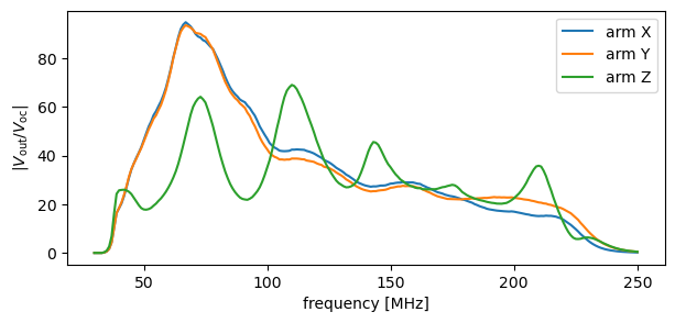
The RF chain’s response 

import matplotlib.pyplot as plt
from grand.sim.detector.rf_chain import RFChain

freqs_mhz = np.arange(30.0, 251.0)
chain = RFChain()
chain.compute_for_freqs(freqs_mhz)
tf = np.abs(chain.get_tf())                        # (arms, frequencies)

fig, ax = plt.subplots(figsize=(7, 3))
for arm, name in enumerate("XYZ"):
    ax.plot(freqs_mhz, tf[arm], label="arm " + name)
ax.set_xlabel("frequency [MHz]")
ax.set_ylabel(r"$|V_{\rm out} / V_{\rm oc}|$")
ax.legend()
plt.show()

Galactic noise at a sidereal time 

One realization of the noise spectrum at the open-circuit terminals, for four units at 6 h local sidereal time:

from grand.sim.noise.galaxy import galactic_noise

spectrum = galactic_noise(6.0, 2048, freqs_mhz, nb_ant=4, seed=0)
print("shape (units, arms, frequencies):", spectrum.shape)

shape (units, arms, frequencies): (4, 3, 221)

du_type selects the antenna model ('GP300', 'GP300_nec', 'GP300_mat').

The T1 trigger 

Apply the offline T1 trigger to the ADC traces of an event:

from grand.dataio import TADC
from grand.sim.detector.trigger import t1_du_triggers

with TADC(str(SAMPLE / "adc_1618-13790_L1_0000.root")) as tadc:
    tadc.get_entry(0)
    counts = np.asarray(tadc.trace_ch)             # (units, channels, samples)

passed = t1_du_triggers(counts)
print("%d of %d units pass T1" % (passed.sum(), len(passed)))

2 of 44 units pass T1

Parameters are passed as a dictionary, for example t1_du_triggers(counts, {"th1": 120}). On noise-free simulations the defaults pass few units; see The offline T1 trigger passes few units on clean simulations.

The arrival direction from peak times 

A plane-wave fit to the times at which the field peaks at each antenna:

from scipy.signal import hilbert
from grand.analysis.fitting.plane_wave import PWF_semianalytical
from grand.dataio import TEfield, TShower

with TRun(str(SAMPLE / "run_1_L0_0000.root")) as trun:
    trun.get_entry(0)
    position = dict(zip(trun.du_id, np.asarray(trun.du_xyz)))

with TEfield(str(SAMPLE / "efield_1618-13790_L0_0000.root")) as tefield:
    tefield.get_entry(0)
    du_id = list(tefield.du_id)
    traces = np.asarray(tefield.trace)              # (units, 3, samples), µV/m
    t0_s = (np.asarray(tefield.du_seconds, dtype=float) - tefield.du_seconds[0]
            + np.asarray(tefield.du_nanoseconds) * 1e-9)

envelope = np.abs(hilbert(traces, axis=-1)).max(axis=1)
t_peak_s = t0_s + 0.5e-9 * envelope.argmax(axis=1)  # 0.5 ns per sample
xants = np.array([position[d] for d in du_id])

theta, phi = PWF_semianalytical(xants, t_peak_s)    # radians
with TShower(str(SAMPLE / "shower_1618-13790_L0_0000.root")) as tshower:
    tshower.get_entry(0)
    print("fit:        zenith %.2f deg, azimuth %.2f deg" % (np.degrees(theta), np.degrees(phi)))
    print("simulated:  zenith %.2f deg, azimuth %.2f deg" % (tshower.zenith, tshower.azimuth))

fit:        zenith 79.70 deg, azimuth 311.53 deg
simulated:  zenith 79.43 deg, azimuth 310.00 deg

The reconstruction works in seconds and radians. Notebook 11 continues with the spherical-wave fit, the amplitude fit and the energy estimate.

Where next 

Tutorial notebooks for each of these tasks at length, with figures.
Command-line tools to run the simulation chain from the shell.
API reference for every function and its arguments.