Tutorial: one shower, start to finish

This tutorial follows one simulated air shower through GRANDlib: from the electric field at the antennas to the voltages, the ADC counts and the trigger, then back from the recorded signals to the direction the shower came from, which it compares with the truth. It takes about fifteen minutes to read and runs in under a minute. You need a working installation (Installation and requirements); the Quick start guide introduces the same calls more briefly.

Every block runs as written, in order, when this page is built.

1. The shower 

The repository includes a ZHAireS simulation converted by sim2root. Its shower tree holds the truth we will try to recover:

import tempfile
from pathlib import Path

import numpy as np
import matplotlib.pyplot as plt
import grand
from grand.dataio import TRun, TShower

SAMPLE = (Path(grand.__file__).parents[1]
          / "sim2root/Common/sim_Xiaodushan_20221026_000000_RUN1_CD_ZHAireS_0000")
EVENT, RUN = 13790, 1

with TShower(str(SAMPLE / "shower_1618-13790_L0_0000.root")) as tshower:
    tshower.get_event(EVENT, RUN)
    true_zenith, true_azimuth = tshower.zenith, tshower.azimuth
    core = np.asarray(tshower.shower_core_pos)
    print("primary %s, %.2g GeV" % (tshower.primary_type, tshower.energy_primary))
    print("comes from zenith %.2f deg, azimuth %.2f deg" % (true_zenith, true_azimuth))
    print("core at x = %.0f m, y = %.0f m" % (core[0], core[1]))

with TRun(str(SAMPLE / "run_1_L0_0000.root")) as trun:
    trun.get_entry(0)
    position = dict(zip(trun.du_id, np.asarray(trun.du_xyz)))   # m, x north, y west

primary 2212, 3.9e+09 GeV
comes from zenith 79.43 deg, azimuth 310.00 deg
core at x = 6217 m, y = 3102 m

A proton of about 4 EeV arriving 79° from the zenith: nearly horizontal, as the showers GRAND is built for. Positions are in meters in the array frame, x toward north and y toward west (Coordinates and conventions).

2. Voltages at the antennas 

Efield2Voltage projects the field on each antenna arm, adds Galactic noise and applies the RF chain:

from grand import Efield2Voltage
from grand.dataio import TVoltage

out = Path(tempfile.mkdtemp())
sim = Efield2Voltage(str(SAMPLE), "voltage.root", output_directory=str(out),
                     seed=7, efield_level=0)
sim.compute_voltage()

with TVoltage(str(out / "voltage.root")) as tvoltage:
    tvoltage.get_event(EVENT, RUN)
    du_id = np.asarray(tvoltage.du_id)
    voltage = np.asarray(tvoltage.trace)                      # µV, (units, arms, samples)
    t0_s = (np.asarray(tvoltage.du_seconds, dtype=float) - tvoltage.du_seconds[0]
            + np.asarray(tvoltage.du_nanoseconds) * 1e-9)    # trace start, s

print("%d units, traces of %d samples at 2 GHz" % voltage.shape[::2])

44 units, traces of 8192 samples at 2 GHz

Each unit’s trace starts at its own time, t0_s, relative to the first unit. Times matter here: the direction is read from when the pulse reaches each antenna.

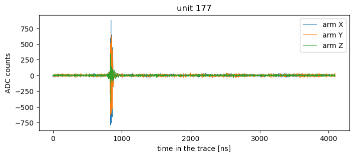
3. ADC counts 

The ADC samples at 500 MHz with 14 bits:

from grand import ADC

adc = ADC()
counts = adc.process(adc.downsample(voltage, 2000.0))      # 2000 to 500 MHz; (units, 3, samples)
dt_ns = 1e3 / adc.sampling_rate                            # 2 ns per sample

loudest = np.abs(counts).max(axis=(1, 2)).argmax()
t_ns = dt_ns * np.arange(counts.shape[2])
fig, ax = plt.subplots(figsize=(8, 3))
for arm, name in enumerate("XYZ"):
    ax.plot(t_ns, counts[loudest, arm], lw=0.8, label="arm " + name)
ax.set_xlabel("time in the trace [ns]")
ax.set_ylabel("ADC counts")
ax.set_title("unit %d" % du_id[loudest])
ax.legend()
plt.show()

4. The trigger 

GRAND’s first-level trigger, T1, decides from each unit’s own trace whether it records the event:

from grand.sim.detector.trigger import t1_du_triggers

passed = t1_du_triggers(counts)
print("%d of %d units pass T1 with the default parameters" % (passed.sum(), len(passed)))

1 of 44 units pass T1 with the default parameters

Very few. The offline T1 rejects most clean simulated pulses, for reasons the trigger group has yet to settle (The offline T1 trigger passes few units on clean simulations). For this tutorial we select units by their signal-to-noise ratio instead.

5. Signal, noise and peak times 

The noise level comes from the start of each trace, before the pulse; the peak time from the maximum of the Hilbert envelope, summed over the three arms:

from scipy.signal import hilbert

noise = counts[:, :, :200].std(axis=2)                       # per unit and arm
snr = (np.abs(counts).max(axis=2) / noise).max(axis=1)        # best arm of each unit

envelope = np.sqrt((np.abs(hilbert(counts.astype(float), axis=-1)) ** 2).sum(axis=1))
t_peak_s = t0_s + dt_ns * 1e-9 * envelope.argmax(axis=1)

print("signal-to-noise above 10: %d units; above 5: %d units"
      % ((snr > 10).sum(), (snr > 5).sum()))

signal-to-noise above 10: 13 units; above 5: 18 units

6. The arrival direction 

A plane-wave fit to the peak times gives the direction the shower came from. It works in meters, seconds and radians:

from grand.analysis.fitting.plane_wave import PWF_semianalytical

xants = np.array([position[d] for d in du_id])

for cut in (10, 5):
    use = snr > cut
    theta, phi = PWF_semianalytical(xants[use], t_peak_s[use])
    print("SNR > %2d, %2d units: zenith %.2f deg, azimuth %.2f deg"
          % (cut, use.sum(), np.degrees(theta), np.degrees(phi)))
print("truth:              zenith %.2f deg, azimuth %.2f deg" % (true_zenith, true_azimuth))

SNR > 10, 13 units: zenith 79.74 deg, azimuth 310.33 deg
SNR >  5, 18 units: zenith 83.84 deg, azimuth 317.50 deg
truth:              zenith 79.43 deg, azimuth 310.00 deg

With the strong units only, the fit recovers the direction to a few tenths of a degree. Lowering the cut to 5 adds units whose largest peak is noise, not the shower. One of them is microseconds away from the front and pulls the answer off by several degrees. A fit is only as good as the units it is given; weighting by timing uncertainty (sigma) or rejecting outliers is the next step in a real analysis.

7. The footprint 

Where the signal is strong shows the shape of the radio footprint. The horizontal axis is east (minus y), so the map reads like a map:

peak_uv = np.abs(voltage).max(axis=(1, 2))
order = np.argsort(peak_uv)

fig, ax = plt.subplots(figsize=(6, 5))
dots = ax.scatter(-xants[order, 1] / 1e3, xants[order, 0] / 1e3, c=peak_uv[order] / 1e3,
                  s=60, cmap="viridis")
ax.plot(-core[1] / 1e3, core[0] / 1e3, "r*", ms=14, label="shower core")

# The shower travels toward azimuth + 180 deg; its ground projection, from the core
travel = np.radians(true_azimuth + 180.0)
ax.annotate("", xy=(-(core[1] + 3e3 * np.sin(travel)) / 1e3, (core[0] + 3e3 * np.cos(travel)) / 1e3),
            xytext=(-core[1] / 1e3, core[0] / 1e3), arrowprops=dict(arrowstyle="->", color="r"))
ax.set_xlabel("east [km]")
ax.set_ylabel("north [km]")
ax.set_aspect("equal")
ax.legend(loc="lower right")
fig.colorbar(dots, label="peak voltage [mV]")
plt.show()

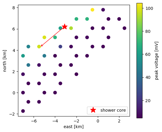
The arrow shows the direction the shower travels. At this zenith angle the footprint is stretched along it over several kilometers, which is why a sparse array can detect very inclined showers.

Where next 

Recipes for each of these steps on its own.
Notebook 11 (Tutorial notebooks) for the spherical-wave and amplitude fits, which also give the distance to the shower maximum and an energy estimate.
The simulation chain for what each stage of the simulation computes.