Validation

How far can GRANDlib’s numbers be trusted? This page shows the checks that compare GRANDlib with something independent of it: a calculation done another way, the shower codes’ own output, or a property that must hold exactly. Each figure and table is computed when this page is built, with the same code the test suite runs (Test suite).

What is not checked here is as important: GRANDlib cannot verify the inputs it is given, such as the sky model, the measured S-parameters or the simulated antenna response. It verifies that it uses them correctly.

Galactic noise against the tables 

The noise level is predicted independently of galactic_noise(), from the shipped power tables and the antenna impedance alone (\(V^2 = 4 P_L \mathrm{Re}(Z)\,\Delta f\), summed over 30 to 250 MHz). The figure compares it with the RMS of the simulated noise over a sidereal day:

from grand import grand_add_path_data
from grand.sim.noise.galaxy import galactic_noise
from tests.sim.test_galactic_noise_normalisation import (
    BIN_WIDTH_HZ, FREQS_MHZ, N_SAMPLES, Z_ANT_FILE)

zant = np.loadtxt(grand_add_path_data(Z_ANT_FILE), delimiter=",", skiprows=1)
r_ant = np.column_stack([zant[:, 1], zant[:, 3], zant[:, 5]])        # Re(Z) per arm
table = np.load(grand_add_path_data("noise/galactic_PL_per_Hz_gp13_GP300.npy"))

lst = np.arange(0.0, 24.0, 1.0)
predicted, simulated = [], []
for hour in lst:
    power = table[:, int(hour * 3), :]                  # 20-minute bins
    predicted.append(np.sqrt((4.0 * power * BIN_WIDTH_HZ * r_ant).sum(axis=0)) * 1e6)
    band = galactic_noise(hour, N_SAMPLES, FREQS_MHZ, nb_ant=200, seed=int(hour))
    full = np.zeros((200, 3, N_SAMPLES // 2 + 1), dtype=complex)
    full[:, :, 30:251] = band
    simulated.append(np.fft.irfft(full, n=N_SAMPLES, axis=-1).std(axis=(0, 2)))
predicted, simulated = np.array(predicted), np.array(simulated)

fig, ax = plt.subplots(figsize=(7, 3.5))
for arm, name in enumerate("XYZ"):
    line, = ax.plot(lst, predicted[:, arm], lw=1.5, label="arm %s, from the tables" % name)
    ax.plot(lst, simulated[:, arm], "o", ms=4, color=line.get_color(),
            label="arm %s, simulated" % name)
ax.set_xlabel("local sidereal time [h]")
ax.set_ylabel("noise RMS [µV]")
ax.legend(fontsize=8, ncol=2)
plt.show()
print("largest difference: %.2f%%" % (100 * np.abs(simulated / predicted - 1).max()))

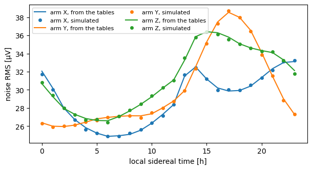
largest difference: 1.13%

The two agree within the statistical spread of 200 simulated units, about 1%, at every hour and on every arm.

The direction of a shower 

A shower’s zenith and azimuth name the direction it comes from. GRANDlib’s spherical transform, applied to the position of the shower maximum that ZHAireS reports, gives back the angles ZHAireS states, for both committed simulations:

from grand.geo.coordinates import _cartesian_to_spherical
from tests.geo.test_angle_convention import SRY, _read

print("%-28s %18s %18s" % ("simulation", "stated (deg)", "from Xmax (deg)"))
for path in SRY:
    zenith, azimuth, xyz = _read(path)
    theta, phi, _ = _cartesian_to_spherical(*xyz)
    print("%-28s %8.2f %8.2f   %8.2f %8.2f"
          % ("_".join(path.parent.name.split("_")[-5:]), zenith, azimuth,
             float(np.ravel(theta)[0]), float(np.ravel(phi)[0]) % 360))

simulation                         stated (deg)    from Xmax (deg)
Proton_3.87_79.4_310.0_13790    79.43   310.00      79.43   310.00
Proton_3.8_51.6_135.4_1618      51.64   135.44      51.64   135.44

ZHAireS prints angles to two decimals and positions to ten meters, which bounds the agreement.

Which arm is which 

The NEC and MATLAB antenna tables name their arms X and Y; the HFSS tables name theirs south-north and east-west. Correlating each response pattern with the HFSS ones, over 60 to 200 MHz, identifies them. The correlations use every fourth azimuth and every second zenith angle, to keep the build fast; the test suite uses all of them:

from tests.sim.test_antenna_arm_identity import _correlation, _pattern

def pattern(name):
    freq, magnitude = _pattern(name)
    return freq, magnitude[:, ::4, ::2, :]

hfss = {"south-north": pattern("Light_GP300Antenna_SNarm_leff.npz"),
        "east-west": pattern("Light_GP300Antenna_EWarm_leff.npz")}
print("%-8s %12s %12s" % ("table", *hfss))
for model in ("nec", "mat"):
    for arm in "XY":
        other = pattern("Light_GP300Antenna_%s_%sarm_leff.npz" % (model, arm))
        print("%-8s %12.3f %12.3f" % ("%s %s" % (model, arm),
                                     *(_correlation(other, h) for h in hfss.values())))

table     south-north    east-west
nec X           0.725       -0.171

nec Y          -0.165        0.655
mat X           0.718       -0.123

mat Y          -0.138        0.623

X correlates with the south-north arm and Y with the east-west arm, in both models. GRANDlib reads them that way; the Handbook has them swapped (The Handbook has the X and Y antenna arms swapped).

Reconstructing a known direction 

Plane waves from 300 random directions, recorded by 30 antennas with a timing uncertainty of 5 ns, are fitted with PWF_semianalytical():

from grand.analysis.fitting.plane_wave import PWF_model, PWF_semianalytical

rng = np.random.default_rng(1)
xants = np.column_stack([rng.uniform(-3000, 3000, 30), rng.uniform(-3000, 3000, 30),
                         1264.0 + rng.normal(0, 20, 30)])
errors = []
for _ in range(300):
    theta, phi = np.radians(rng.uniform(50, 88)), np.radians(rng.uniform(0, 360))
    times = PWF_model((theta, phi), xants) + rng.normal(0, 5e-9, 30)
    fit = np.array(PWF_semianalytical(xants, times))
    true = np.array([np.sin(theta) * np.cos(phi), np.sin(theta) * np.sin(phi), np.cos(theta)])
    got = np.array([np.sin(fit[0]) * np.cos(fit[1]), np.sin(fit[0]) * np.sin(fit[1]),
                    np.cos(fit[0])])
    errors.append(np.degrees(np.arccos(np.clip(true @ got, -1, 1))))

fig, ax = plt.subplots(figsize=(6, 3))
ax.hist(errors, bins=30)
ax.set_xlabel("angle between fitted and true direction [deg]")
ax.set_ylabel("directions")
plt.show()
print("median error %.3f deg, 95%% below %.3f deg"
      % (np.median(errors), np.percentile(errors, 95)))

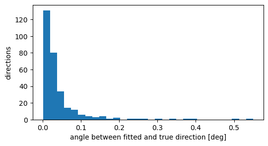
median error 0.022 deg, 95% below 0.149 deg

This checks the fit against its own model: real showers have curved fronts and less regular timing, which the Tutorial: one shower, start to finish shows on a simulated one.

Properties that hold exactly 

Some checks need no reference at all:

The noise spectrum and the noise trace carry the same power (Parseval’s theorem), to \(10^{-9}\).
Converting a position between frames and back returns it unchanged.
The same seed gives the same noise; a different one does not.
The cascade of a matched, lossless line is the identity matrix.

Regression checks 

Two further checks show that the answer has not changed, not that it is right. tests/sim/test_pipeline_golden.py runs the whole chain on a fixed input and seed and compares the result with a stored reference, to \(10^{-6}\) of the trace peak. tests/dataio/test_schema_snapshot.py compares the layout of every ROOT tree with a stored snapshot. A change to either appears in review.

Where next 

Test suite for the whole test suite.
Known issues for what is known to be wrong or undecided.
Notebook 05 (Tutorial notebooks) for the Galactic noise in detail.

Validation

Galactic noise against the tables

The direction of a shower

Which arm is which

Reconstructing a known direction

Properties that hold exactly

Regression checks

Where next